Advanced example

This guide shows how to analyze real images jointly. It is recommended to start off with the Quickstart Tutorial before engaging in this example. The dataset consists of a MALDI and optical images of mouse urinary bladder. These are processed images from original images downloaded from PRIDE (dataset id PXD001283).

The images are located in the data/Mouse_Urinary_Bladder_PXD001283/ directory: ms_image_resized.imzML, optical_image.tiff.

We aim at finding the spatial correlations between the ion images in MALDI and the optical image.

Data processing

The following section explains how the images were processed from the original images available from PRIDE. It is not necessary to replicate these steps, but they are detailed for reproducibility purposes. Jump straight to Fusion workflow if you wish to get started with this example.

The original MALDI image from PRIDE has different m-z values. First, all spectra are aligned on the same m/z-axis following the procedure described in the Data section (parameters: factor=150, level=2, nbpeaks=1, step=0.02). Then, the images are resized using the examples/resize_imzml.py script with a 0.5 scale factor.

Peak selection and alignment are already done, thus there is no need for further spectra processing.

In essence, the following scripts were applied. First, we download the data from PRIDE:

cd data/Mouse_Urinary_Bladder_PXD001283/
python download.py

After completion (might take a while), the three following downloaded files should be located in the data/Mouse_Urinary_Bladder_PXD001283: ms_image.imzML, ms_image.imzML, and optical_image.tiff.

Next, we align and resize the image:

cd ../../
python -m examples.same_mz_axis -i data/Mouse_Urinary_Bladder_PXD001283/ms_image.imzML -o data/Mouse_Urinary_Bladder_PXD001283/ms_image_aligned.imzML -f 150 -l 2 -n 1 -s 0.02
python -m examples.resize_imzml -i data/Mouse_Urinary_Bladder_PXD001283/ms_image_aligned.imzML -o data/Mouse_Urinary_Bladder_PXD001283/ms_image_resized.imzML -f 0.5

The optical image is transformed by a 5° counter-clockwise rotation followed by a +100 px translation on the x-axis and a scaling by a factor of 0.9.

Fusion workflow

Let’s import the necessary modules and define some utility functions:

%load_ext autoreload
%autoreload 2

import sys, os
import matplotlib
import matplotlib.pyplot as plt
import numpy as np
import string
import SimpleITK as sitk

rootpath = "../../"
imagepath = "data/Mouse_Urinary_Bladder_PXD001283/"
sys.path.append(os.path.join(os.path.dirname(os.path.abspath("__file__")), rootpath))

def display_image(image):
    plt.axis("off")
    plt.imshow(image, cmap="gray")
    plt.show()

def display_images(*images):
    fig, ax = plt.subplots(1, len(images))
    for i in range(len(images)):
        ax[i].axis('off')
        ax[i].imshow(images[i], cmap="gray")
        ax[i].text(0.4, -0.2, "(" + string.ascii_lowercase[i] + ")", transform=ax[i].transAxes, size=18)
    plt.show()

Input, Visualization

The data is available in the data/Mouse_Urinary_Bladder_PXD001283 directory. First, read the data and display the spectrum of a pixel:

import esmraldi.imzmlio as io

imzml = io.open_imzml(rootpath + imagepath + "ms_image_resized.imzML")
spectra = io.get_spectra(imzml)

print(spectra.shape)
mz_first, intensities_first = spectra[1, 0], spectra[1, 1]
indices = intensities_first > 1
plt.stem(mz_first[indices], intensities_first[indices], use_line_collection=True)
plt.show()

(8711, 2, 214)

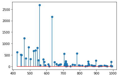
The variable spectra is a 3D numpy array, with 8711 pixels (67x130) and where each pixel is associated to a spectrum with 214 peaks. The peaks are already selected and aligned for this dataset.

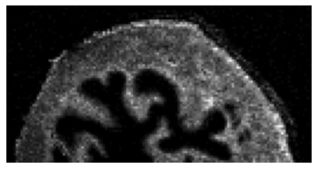
Then, we display the image of the ion of m/z 741.7 +/- 0.25:

image = io.get_image(imzml, 741.7, 0.25)
display_image(image)

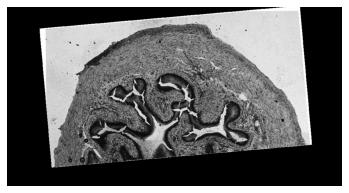
Now, we read the optical image:

from skimage import io as skio

optical_image = skio.imread(rootpath + imagepath + "optical_image.png", as_gray=True)
display_image(optical_image)

Segmentation

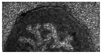
Next, a representative image is extracted from the set of MALDI ion images. This is achieved by region growing on a subset of relevant images, i.e. non-noisy images.

Relevant images are found by the spatial coherence measure.

import esmraldi.segmentation as seg

maldi_image = io.to_image_array(imzml)
maldi_image = np.transpose(maldi_image, (1, 0, 2))
maldi_image = io.normalize(maldi_image)

# Relevant images
spatially_coherent = seg.find_similar_images_spatial_coherence(maldi_image, 300, quantiles=[60, 70, 80, 90])

# Mean image
mean_image = np.average(spatially_coherent, axis=-1)

# Region growing
seeds = set(((1, 1), (0, 0)))
list_end, _ = seg.region_growing(spatially_coherent, seedList=seeds, lower_threshold=30)
x = [elem[0] for elem in list_end]
y = [elem[1] for elem in list_end]
mask = np.ones_like(mean_image)
mask[x, y] = 0
segmented_image = np.ma.array(mean_image, mask=mask)
segmented_image = segmented_image.filled(0)

display_image(segmented_image)

Registration

At this stage, both shapes in the optical and MALDI images can be matched. In our case, we register the MALDI segmented image onto the optical image.

import esmraldi.registration as reg
import esmraldi.imageutils as utils

segmented_itk = sitk.Cast(sitk.GetImageFromArray(segmented_image), sitk.sitkFloat32)
optical_itk = sitk.Cast(sitk.GetImageFromArray(optical_image), sitk.sitkFloat32)
segmented_itk = utils.resize(segmented_itk, optical_itk.GetSize())
segmented_itk = sitk.Cast(segmented_itk, sitk.sitkFloat32)

number_bins = 8
sampling_percentage = 0.1
registration = reg.register(optical_itk, segmented_itk, number_bins, sampling_percentage, seed=0, learning_rate=0.8, relaxation_factor=0.8, min_step=0.0001)
registered_seg_itk = registration.Execute(segmented_itk)
registered_seg_image = sitk.GetArrayFromImage(registered_seg_itk)

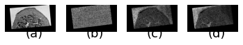
display_images(optical_image, segmented_image, registered_seg_image)

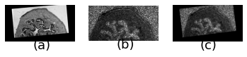
(a⁣) Optical fixed image, (b) original MALDI segmented image and (c) registered MALDI image.

Finally, we apply the registration to the original MALDI image:

registered_itk = sitk.GetImageFromArray(maldi_image)
registered_itk = utils.resize(registered_itk, optical_itk.GetSize())
registered_itk = sitk.Cast(registered_itk, sitk.sitkFloat32)
size = registered_itk.GetSize()

size = [size[1], size[2], size[0]]
out_register = sitk.Image(size, registered_itk.GetPixelID() )

for i in range(registered_itk.GetSize()[0]):
    slice = registered_itk[i, :, :]
    slice.SetSpacing(optical_itk.GetSpacing())
    slice_registered = registration.Execute(slice)
    slice_registered = sitk.JoinSeries(slice_registered)
    out_register = sitk.Paste(out_register, slice_registered, slice_registered.GetSize(), destinationIndex=[0, 0, i])

registered_image = np.transpose(sitk.GetArrayFromImage(out_register), (1, 2, 0))

Joint statistical analysis

The final step of the workflow is to find the MALDI ion images whose distribution correlate with the optical image.

We use non-negative matrix factorization (NMF) to find spatial correlations.

We search for the 3 ion images which are closest to the optical image:

import esmraldi.fusion as fusion

optical_flatten = fusion.flatten(optical_image).astype(np.float32)
maldi_flatten = fusion.flatten(registered_image, is_spectral=True)

# Reduction by NMF
mzs = spectra[0, 0, :]
fit_red = fusion.nmf(maldi_flatten, n=5)
reduction = fit_red.transform(maldi_flatten)
point_optical = fit_red.transform(optical_flatten)
weights = [1 for i in range(reduction.shape[1])]

similar_images, similar_mzs, distances = fusion.select_images(registered_image, point_optical, reduction, weights, mzs, labels=None, top=None)

print("Closest m/z ratio ", similar_mzs[:3])
display_images(optical_image, similar_images[..., 0], similar_images[..., 1], similar_images[..., 2])

[[3.3571892 2.3540816 0.4886422 2.3008347 0.991761 ]]
Closest m/z ratio  [686.57623549 492.95937632 559.01787735]